Program Visualization as Abstract Interpretation
For this past semester, I’ve been thinking in a semi-principaled way about how we should visualize program executions. For example, how should we visualize this program:
let id x = x in
let g x = id x
let check_zero y = if y = 0 then bad () else 1
if (y >= 0) check_zero (g y) else h y
Let’s say we want to check whether or not bad is ever called: and if
so under what circumstances The most intuitive way we could do this is
obviously to just sit and think about the program: the program will
call bad exactly when y is zero.
For small programs like these, checking things like this are easy enough, even if the control flow is a little convoluted. As programs get larger, it’s harder and harder to convince ourselves that these properties are correct: so we build tools to do it for us. One of the most basic tools we can use is a test-suite and a debugger. The programmer will provide a set of sample inputs to test these inputs on, and will visualize them as they go.
With a debugger, we can see exactly when the call to bad happens by
“focusing” in on a single run of the program where y is zero. But
what if we have a bunch of runs of the program and we want to see
what sorts of functions are called by it, perhaps because we’d like to
get some understanding of what the program does? For example, let’s
say that we wanted to see what happens to the program when y is 0
and when y is 1.
We could use our debugger for each of those paths, but clearly as the programs get large, introspecting program behavior like is going to start to become very tedious. And this is the crux of my post:
We can use tools from abstract interpretation to guide us in constructing program visualizations.
Namely: we’re going to think about a debugger as something that
produces “steps” of the program execution, and then we’re going to
construct a graph of the program that will summarize what the program
is doing to a viewer. Because we want this graph to summarize a bunch
of executions, we’re going to collapose certain parts of the graph
(perhaps each invocation of f in this program, perhaps) so that they
can be more easily viewable by a user. Then, we’re going to make it
interactive, so that when the user wants more information they can
click on a node and disambiguate that node based on its context.
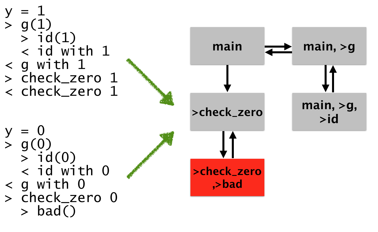
For example, here’s a mockup of what this might look like after we’re done:
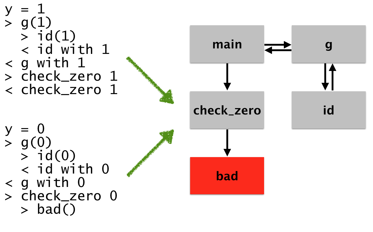
On the left are two runs of the program. In the first, we start with
y = 1, we then call (the > designate entries) g, which
subsequently calls id, returns to g (with 1 as the return
value), and then calls check_zero. In the other run, we see the same
thing, except with the bad behavior.
In this case, the logs we see on the left represent a subset of the actual program behavior, so the facts we get to check are up to the granularity of the information given in these logs. What I want to do in this blog post is to convince you that visualizing dynamic runs in this way can be aided by coalescing this dynamic information into a graph-based representation, and then be disambiguated by interacting with that graph.
This summary seems like a nice idea, but it doesn’t actually allow us
to see what really happened in the program: it just shows us a control
flow graph. We know that bad was called, but not under what
condtiions. Similarly, we might like to find out under what conditions
our various functions (like g and id) were called. To do this,
we’re going to have this behavior: whenever you click on a various
node, you’re going to be able to see (in another view) which points in
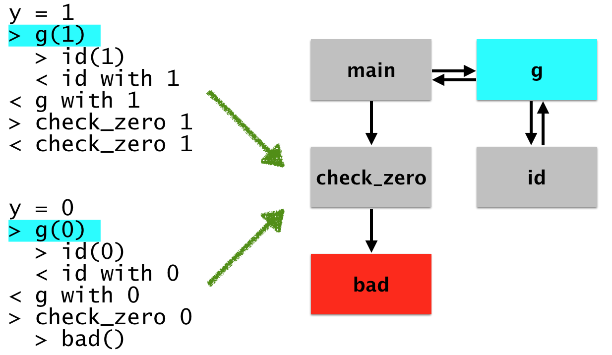
each run correspond to that node. For example, let’s say you want to
know all of he possible places that g was called from. You click on
it, and then our visualizer will tell you which lines in the program
actually corresponded to that invocation. Like so:
Let’s say that you want to introspect here, you might want to just “focus in” on the bad log. To do that, you’ll just project out the operation of building the graph. You can even build a more finely grained graph which shows precise call / return structure:
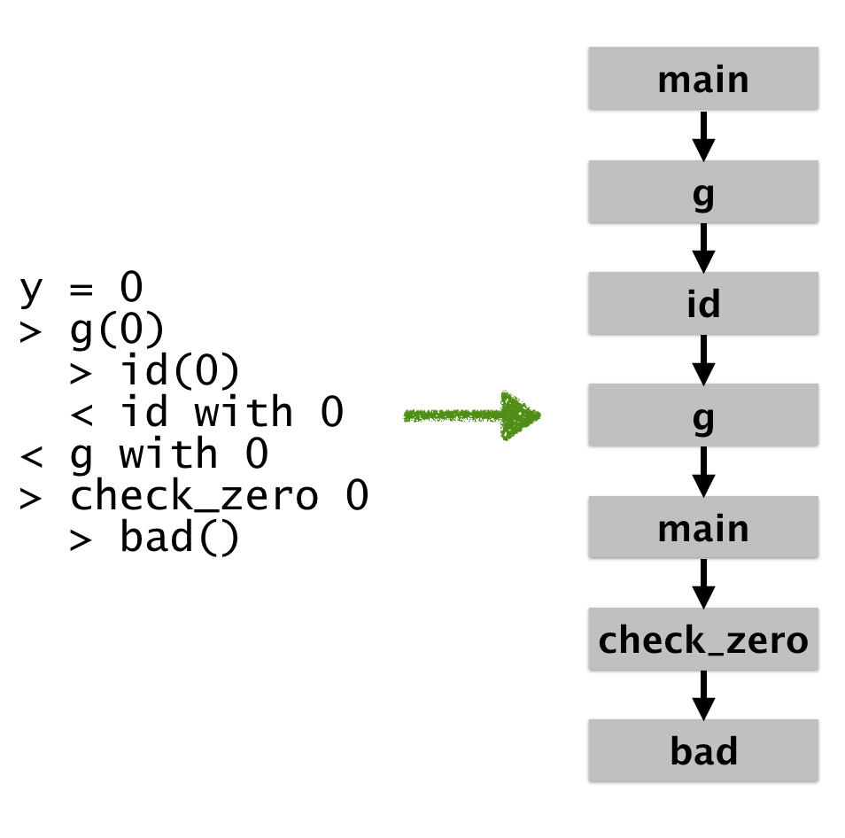
The last execution graph is obviously the most precise. It shows exact
call/return sequences in a finely grained way. If we were to formalize
it, the concrete states would differ: the first g represents the
entry while the second represents something like the exit. But this
precision comes at a cost: it shows us a lot of information that will
probably be meaningless until we really know what we want to look for.
For example, here’s a program with an off by one error:
void traverseList(Link *list) {
  Link *x = list;
  Link *y;
  do {
    x = x->next;                // Line 4
    y = x->next;                // Line 5
  } while (x != null)           // Line 6
  // ...
}
As a high level view of the program, we might make our states function calls with line numbers into the function. A concrete execution would look like:
x = ptr;      // x -> <1,2>
x = x->next   // x -> <1>
y = x->next   // y -> null
x != null
x = x->next   // x -> <null>
y = x->next   // BAD!
Once we isolate the bad thing, we can traverse back to the bad configuration that caused it to happen, perhaps with the aid of (e.g.,) a time traveling debugger such as that in OCaml.
I haven’t yet said how we get these logs, or what the concrete structure of the logs looks like. In this case, we wanted to know about the program’s control flow behavior: when did bad states get reached, or which functions called which others. Because I only cared about the control flow behavior of the program under various circumstances, it was sufficient to include function entries and exits. If I had instead wanted to talk about something more general, I’d have to change what the log looks like. For example, say I wanted to talk about the structure of the heap. I’d have to instead include information in the log about how the heap evolves over time. I’m not particularly concerned with how we get the information here at a technical level, but I’m currently simply instrumenting the program to log method-call sequences. I’m sure you could get useful information via a similar program instrumentation framework like Valgrind or a debugger.
Getting more formal with it
So now that I’ve presented some of this, I’d like to make the case that we can use machinery from abstract interpretation to help us draw these cool graphs. To start off developing the machinery we’ll need for graph, and abstraction, let’s first develop the “most precise” one I discussed above.
First, we need to define a little bit formally what our log looks
like. In this example, the method call sequnce gives us an idea about
the evolution of the program’s control flow. We can think about this
as having our semantics running in an abstract machine, and our log
entries (each individual line of the logs) showing us deltas that
generate new machine states. In other words, log entries represent
transitions from machine states to new machine states. Now, if our log
contains all of the possible information we could need to recover the
concrete execution of the program, we’d end up being able to use our
log entries to perfectly recover the concrete execution of the
program. Let’s say that our log is a list of transitions:
t₁,t₂,...,tᵢ
Let’s assume that we have some type transition that stands for
whatever transitions are. In this example, my type transition would
look like this:
type transition =
  | Entry of name * value list
  | Return of value
Then, formally, each transition would take us from some program state
Σ, to a new state Σ': step : Σ → transition → Σ. Typically, we
designate some initial state Σι that acts as the initial state of
the program. If this is the case, then for any sequence of transitions
t₁,...,tᵢ, we have that the transitive closure of the step relation
with that set of transitions will reach some new program point:
Σι →ᵗ₁ Σ₁ →ᵗ₂ ... → Σᵢ
Now, so far I haven’t put any meaningful stipulations on what the
transition function must look like. I have merely asserted that for it
to be meaningful, we have that there be some definition of program
states Σ and a step relation that operates on states and
transitions. But how do we know that the transition function we have
in mind is actually meaningful? I haven’t worked out all the details,
but I think you basically want some correspondence between derivations
of new states via the step function and the actual semantics for
your program. In other words, you want this to hold: “whenever I
observe that Σι →ᵗ¹⁻ᵗⁱ Σᵢ, I can come up with a derivation in the
semantics that mirrors that set of transitions.”
Now, notice that my transitions here are only giving us partial
information about program states. In reality, this is fine, as long as
they’re giving us enough information to ascertain what we care
about. But formally, it means that our transition relation won’t talk
about the concrete program semantics, it’ll actually be talking about
an abstract semantics. To make this idea more concrete, in my example
logs here, I’ve included the function parameters and return
values. But let’s say I didn’t. Then, when we looked at a line in
the log, say >g, we wouldn’t know what actual parameter g was
called with. Instead, we’d be forced to think that g could have been
called with anything (that the program could have called it with, of
course).
Producing the “most precise” graph
Now that I’ve set up all this machinery, what is the version of this “most precise” graph for our semantics. Here we’ll assume that our transitions have a type like this:
type transition = entry × line number × log number
and entry =
  | Entry of name * value list
  | Exit of value
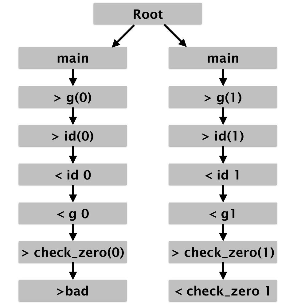
Let’s first define our program states. Our states are literally just
going to be mirrorings of the transitions, except for a special
initial state I designate as Root so that our step function will
then just be the identity. This will give us a forest of possible
configurations (one linear sequence of states for each log).
Σ = log entry × line number × log number + Root
Σᵢ (log_number) = Root
step (_,i,k) (entry) = (entry,i+1,k)
Here’s what it looks like for our two logs shown here:
A control flow analogue
Let’s say that we want to make the first graph above: in that setting we wanted to give a high level view of the program’s control flow, while still allowing the user to disambiguate points in the chart. In other words, we’re trying to find a way to compress the most recent picture – where we show all of the possible “unrolled” behavior – into the first one (that coalesces that behavior).
Since we’re trying to think about control flow problems (“who called what”), it seems sensible to think about the control flow behavior of the runs.
y = 0
> g(0)
  > id(0)
  < id with 0
< g with 0
> check_zero 0
  > bad()
To build up our graph, we’ll start in the “main” function, and then
watch for transitions. For example, upon seeing the >g(0)
transition, we’ll draw a new state g. And then, upon seeing the
>id(0) transition, we’ll draw another new state id. How do we know
where to go when we see the <id transition, however? We want to
return to the caller, but don’t have the information to know where to
return.
The semantics of the program handles this by maintaining a stack of functions. We can do that here:
Σ = frame list
frame = function name
Here, we’re ignoring arguments to functions (our frames don’t maintain environments), but we do get arbitrary context sensitivity as long as we set things up correctly.
Now, we need to define the step function for a single log, and then lift that up to a set of logs. This is pretty simple: when we see an entry we add generate a new state that adds it to the stack, and when we see a return we pop a frame from the stack. We assume that calls and returns are balanced (which would be required by the semantic rules defining soundness I mentioned above).
step Σ (> method)             = method :: Σ
step (method :: Σ) (< method) = Σ
We then take the reflexitive transitive closure of this relation over both of our logs. This graph has as its nodes sequences of call frames (without their arguments / returns), and is isomorphic to the graph in the first example:
Unfortunately, because this style of analysis allows an arbitrarily large permutations of method calling sequences, it allows the graph’s behavior to degrade to a pathological case we want to avoid. For example, consider the factorial function:
let fac n =
  if n = 0 then 1 else fac (n-1)*n
In that graph, we’d see an arbitrarily long chain of fac calls when
our log called the program for some large value of n. Instead of
showing that, let’s say we wanted to only have one occurrence of each
method in the program, and then show arrows between method calls when
there could potentially be control flow between them.
To set this up, we’ll change our state space slightly to mirror a
little bit more of a traditional abstract machine. We’ll get an
isomorphic state space, but we’ll massage the machine a bit so that
it’s easier to abstract things later. Just as before, our state space
will keep track of the current function fn, but now we’ll keep a
pointer to the continuation. That pointer is going to be an address
into a store σ, which has the type Address → Continuation. The
store is just a place through which we thread continuations (in a
linked-list style structure). Continuations are either function names
and addresses, or the special Done continuation (which says there is
nothing else to do). We also need an auxiliary function alloc, which
gives us a fresh address for the store. We will define the step
function to put a new address in the store whenever we see a new stack
frame. The notation σ ⊔ [ a ↦ (fn,k) ] reads, “extend the store σ
with a binding that makes a point to the continuation (fn,k).”
Σ = ⟨ fn, σ, c ⟩
σ : Address → Continuation
Continution = fn , address | Done
c : Address
Σι = ⟨ main, [a₀ ↦ Done], a₀ ⟩

a = alloc (Σ)
step ⟨ fn, σ, c ⟩ (> f) = ⟨ f, σ ⊔ [ a ↦ (fn, k) ], a ⟩
step ⟨ fn, σ, c ⟩ (< f) =
  let fn', c' = σ(κ) in ⟨ fn', σ, c' ⟩
For our example program above, we’d get this:
> g(0)
⟨ g, [a₁ ↦ (main,a₀), a₀ ↦ Done], a₁ ⟩
  > id(0)
  ⟨ id, [a₂ ↦ (g, a₁), a₁ ↦ (main,a₀), a₀ ↦ Done], a₂ ⟩
  < id with 0
  ⟨ g, [a₂ ↦ (g, a₁), a₁ ↦ (main,a₀), a₀ ↦ Done], a₁ ⟩
< g with 0
⟨ main, [a₂ ↦ (id, a₁), a₁ ↦ (main,a₀), a₀ ↦ Done], a₀ ⟩
> check_zero 0
  ⟨ check_zero, [a₃ ↦ (main, a₀, a₂ ↦ (id, a₁), a₁ ↦ (main,a₀), a₀ ↦ Done], a₀ ⟩
  > bad()
  ⟨ bad, [a₄ ↦ (check_zero, a₁),
          a₃ ↦ (main, a₀, a₂ ↦ (id, a₁), a₁ ↦ (main,a₀), a₀ ↦ Done], a₄ ⟩
If you haven’t guessed yet, this machine is an instance of the abstracting abstract machines formulation, and my approach follows theirs.
The last step: abstraction
Now that we’ve rearranged our visualization to use an abstract machine structure, we need to exploit it. Let’s think about what happens to our state space as we add the next log. First, we need to start with the last state from performing our last analysis, and we need to “reset” the analysis into the initial state. But it’s not quite the same initial state: we just want to reset to the start function:
⟨ main, [a₄ ↦ (check_zero, a₁),
         a₃ ↦ (main, a₀, a₂ ↦ (id, a₁), a₁ ↦ (main,a₀), a₀ ↦ Done], a₀ ⟩
y = 1
> g(1)
  ⟨ g, [a₅, (main,a₀), a₄ ↦ (check_zero, a₁),
        a₃ ↦ (main, a₀, a₂ ↦ (id, a₁), a₁ ↦ (main,a₀), a₀ ↦ Done], a₅ ⟩
  ...
Now here, our function alloc returns a fresh address a₅. To get
the behavior, we actually want to reallocate a₁. This means that
our continuations have to be able to store sets of functions, and
sets of next continuations. So instead of our store having the
structure:
σ : Address → Continution
Continution = fn , address | Done
We need to lift continuations to hold sets of functions and addresses. Because they actually represent sets of continuations, we’ll call them abstract continuations (or flow sets, in control flow terminology):
Continution^ = ℘(fn) × ℘(address) | Done
Now, we’re going to have to modify our alloc function to “smush
together” things that come from the same function. We’re going to do
that by changing the structure of addresses (which I’ve so far been
leaving as opaque). Instead, we’re going to make addresss simply
function names:
Address = fn | Done
Now, our allocator is going to be this:
alloc (fn,σ,c) = fn
Last, we have an operation σ ⊔ [ a ↦ (fn,k) ] which we have to make
sense of with our modified notion of continuations. First, we need to
note that it must really be σ ⊔ [ a ↦ {(fn,k)} ]. Then, the join
operator ⊔ will be the natural elementwise distribution over the
sets of functions and continuations.
Mapping between different analyses: insertions
(This is the most hand-wavy section because I haven’t really figured it out yet..)
Alright, so now we have a few different kind of analyses, and I’m convinced that we can generate many, many more. But when we’re visualizing programs, we don’t just want one analysis, we want to mix a few of them together and map between them.
Let’s say that you want to map this 0CFA-continuation-allocator semantics to the “fully unrolled” visualization, like I showed in the second picture. What you do is to run both step functions in sequence, and recognize when you’re coalescing the fine grained states into the abstract states. Doing that, you establish a mapping between the 0CFA thing and the fully precise thing. But in general, I imagine a big interactive tool that allows you to take a set of logs (equivalently: one really big log) and imbue any sort of visualization (or analysis) you want onto it. I think this trick of running the different analyses in parallel can be formalized as Galois insertions, but I haven’t fully worked out the details yet.
For measure, I’m doing this right now in ongoing research: where I map function entries down to the set of concrete points in a “fully precise” (linear) log. The visualizer allows the user to click on function entries and disambiguate based on the places in the log that are being coalesced into that high level node.
Closing notes
The fact that we can use the machinery of abstract machines to think about visualizing program executions is probably unsurprising to many people: concrete executions are, of course, simply instances of abstract executions. However, I think there are a few powerful things that we can take away from this exercise.
First, there are situations in which building an abstract interpreter might be too difficult to do with sufficient precision. Perhaps it’s a new programming language, toolchain, etc.. In these cases, I would guess that it’s easier to dynamically instrument the program to capture the facts you want, and then write a visualization for it post-hoc.
Next, real program runs allow us to “focus in” on the interesting behavior in our program. Concrete executions allow infinite precision (at the cost of soundness). In this post, I’ve set things up so that we can use abstract interpretation machinery to view and understand concrete runs. But I think there’s also room to be able to use these insights to design patterns that allow mixing the concrete and abstract worlds, or even turning the knobs on various analyses. Specifically, I think these ideas could immediately be used to visualize runs of a symbolic executor. Expanding on that, I think a good way to interact with a program analysis is to gradually “peel away” and “focus in” on various parts of the exeuction, in the way that I’ve tried to do here.
Last, thinking about this was interesting for me in that it helped further connect abstract interpretation to something tangible that makes sense to me (debugging a program). When I first learned about abstract interpretation (and still), I was tempted to think about it as something separate from a metaphor that I can easily comprehend: tracking concrete executions.
The upshot of this post is this question: to what extent can we use the abstractions we design for program analysis to also visualize executions of those programs. This is one of the first posts I hope to make on this topic. It came out of wanting to generalize some of the work I’d been doing in visualizing security properties for programs. That being said, I think there’s still a long way to go: defining more concretely what an “instrumentation” is, trying it out for a lot more examples, and applying it to popular program visualization tools (like Python Tutor!). I hope I get a chance to work on this more and flesh some of these ideas out in the future.